





Beam angle and candela distribution are quoted as if they were properties of the LED alone. They are properties of the LED plus the distance at which the measurement was taken. For extended sources the two regimes disagree, and choosing the wrong one produces beam data that does not survive contact with the application.
The Far-Field Condition
Photometric theory assumes a point source. That assumption holds once the detector sits far enough away that the source subtends a negligible angle. The rule of thumb is five to ten times the largest dimension of the emitting area, which defines the far-field distance. A 5mm LED satisfies it at centimeters; a 300mm panel needs 1.5 to 3 meters before its distribution stabilizes.
In the far field, irradiance falls with the square of distance and the angular distribution does not change with distance. Almost every datasheet beam plot you have seen is a far-field plot.
Why Near-Field Exists
Real LED sources are not points. An array, a light guide or a diffuser panel has an emitting area large enough that different parts of the source are at different distances and angles from any nearby detector. At short range the illumination pattern on a surface depends on the shape and radiance distribution of the emitter, not just its total flux.
Near-field photometry measures radiance at many points across the emitting surface, then computes the far field mathematically from that map. One near-field scan, done once, yields the distribution at every distance. This is how lighting simulation tools build models of real luminaires.
| Property | Near-field | Far-field |
|---|---|---|
| Detector distance | Source dimension scale | 5-10x source dimension |
| What is measured | Radiance map of the surface | Angular intensity distribution |
| Valid for | Any distance by computation | That distance regime and beyond |
| Typical tool | Imaging goniophotometer | Standard goniophotometer |
| Fails when | Rarely; expensive setup | Source is large relative to range |
Where the Difference Bites
Three cases make the choice practical rather than academic. Small high-power chips with reflector or lens optics behave as point sources well within a meter, so far-field data is accurate for spotlights and downlights. Large-area panels and linear luminaires measured at one meter in a lab will show a different beam in a real room at working distances; the near-field computation corrects for this. High-bay and streetlight optics mix both regimes, because the optic shapes the beam at the source while the installation distance sits far away.
A practical check: if the datasheet states the measurement distance and it is at least five times the emitting aperture, trust the plot. If it is silent on distance, ask.
Units That Follow the Regime
Far-field data is expressed in candelas, candela per kilolumen or as a polar or cartesian intensity plot. Near-field data starts in luminance, candela per square meter, and produces the far field by projection. Lighting design software consumes IES and LDT files, which are far-field formats; the near-field work happens upstream, at the luminaire maker, to generate those files correctly.
FAQ
Can I just multiply a far-field plot down to close distances? No. The inverse square law only holds in the far field. Below that boundary the predicted illuminance overstates what an extended source actually delivers at close range.
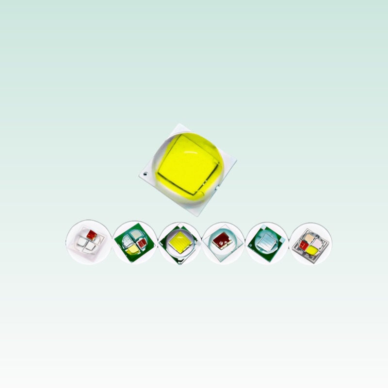
Do COB LEDs avoid the problem? Mostly, yes. Their small emitting diameter means far-field is reached quickly, which is one reason they remain common in focused optics.
Is near-field always better? It is more information, but costlier and slower. For point-like sources it adds nothing over a direct far-field scan.
